behavr tables
A single data structure to store data and metadata
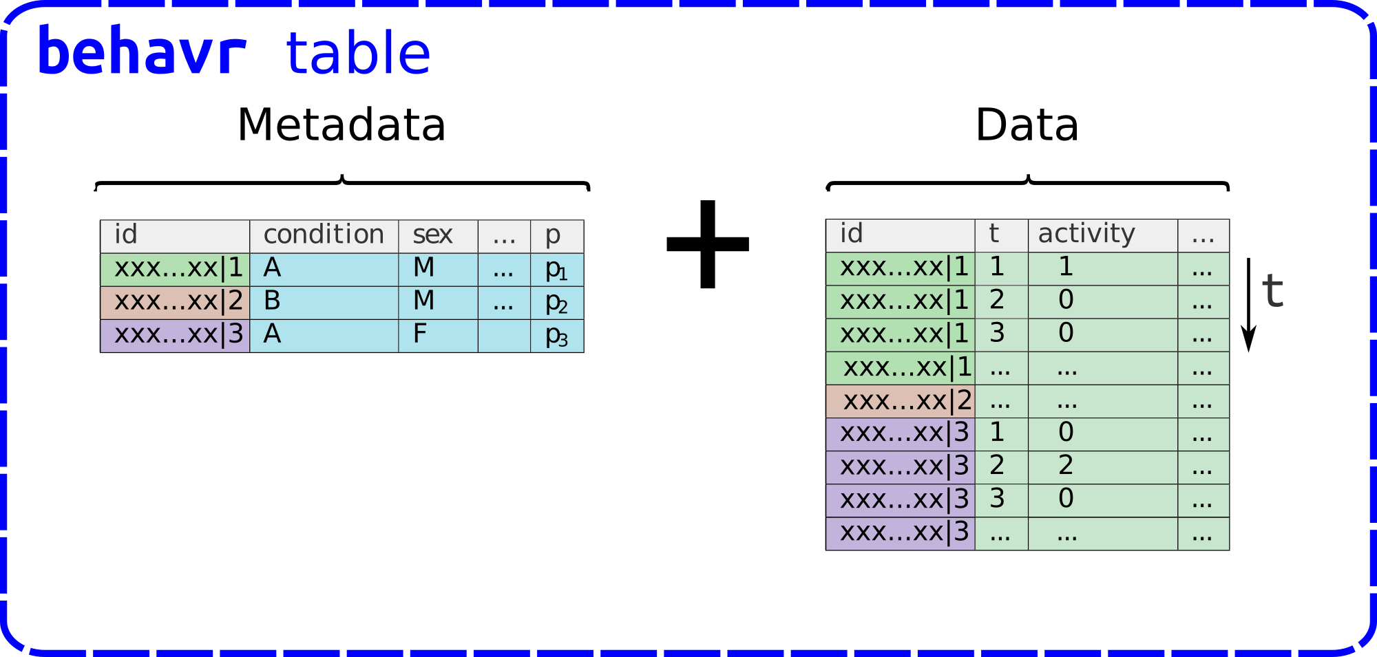
a behavr table
Variables and metavariables
As we have seen in the previous section, metadata are crucial for proper statistical analysis of the experimental data. In the context of ethomics, the data are long time series of recorded variables such as position, orientation and number of beam crosses, for each individual.
Variables are different form metavariables in so far as the latter are made of only one value per animal.
It is easier (and less error prone) to always keep the data and metadata together.
In rethomics, in order to handle large amounts of data (together with metadata), we have designed the behavr package.
behavr tables are based on the very powerful package data.table, but enhanced with metadata.
A behavr table is, indeed, formed internally by two tables: the metadata table and the data table, both are linked by the id column (see figure above).
For most purposes, you can use a behavr table just like a data.table.
Therefore, do take a look at the introduction to data.table for further details!
When we load any behavioural data in rethomics, we get a behavr table as a result.
In this section, we will discuss the usual operations that you can perform on behavr tables.
Operating on behavr tables
Now that we have all our data at the same place, we want to be able to manipulate it.
In the next part of this tutorial, we will create some toy data and learn how to manipulate it.
This is where basic knowledge of data.table comes in handy.
The following table is an overview of operations in behavr tables.
DT represents an behavr table.
| Section | Operation | Expression | Example |
|---|---|---|---|
| Generalities | Summarise behavr table |
summary(DT) |
How many individuals, variables, metavariables, etc? – summary(dt) |
| Pure data | Create/alter a variable | DT[, new_column := some_value] |
When are animals ‘very active’? – dt[, very_active := activity >= 2] |
| Remove a variable | DT[, column_to_delete := NULL] |
Lets remove a variable we don’t need? – dt[, very_active := NULL] |
|
| Select data rows | DT[criteria] |
Exclude data before the first hour – small_dt <- dt[t > hours(1)] |
|
| Pure metadata | Access metadata table | DT[meta = TRUE] |
Show metadata as table – dt[meta = TRUE] |
| Create/alter metavariable | DT[, new_meta := some_value, meta=TRUE] |
Define a new factor that is a comibiation of ‘sex x condition’ – dt[, treatment := paste(sex, condition, sep='|'), meta=T] |
|
| Meta & data | Use metavariable as variable | xmv(metavariable) |
Add 10s to all time, only for animals in condition 'A' – dt[, t := ifelse(xmv(condition) == 'A', t + 10, t)] |
| Remove individuals according to metavariable | DT[criteria] |
Remove all males (from data, and metadata) – dt_females <- dt[xmv(sex) == 'females'] |
|
| Summarise | Compute individual statistics | DT[, .( statistics = some_math()), by='id'] |
Compute the average activity, per animal – stat_dt <- dt[, .(mean_acti = mean(active)), by='id'] |
| Rejoin metadata to data | rejoin(DT) |
Merge metadata and summary statistics – stat_dt <- rejoin(stat_dt) |
|
| Advanced | Stitch experiments | stitch_on(DT, metavariable) |
TODO – TODO |
Playing with toy data
The behavr package has a set of functions to make toy data. This provides us with a playgound to test functions and plots without having to get any real data.
In order to understand behavr object, lets create a toy one.
First, we make some dummy metadata (always needed to create a behavr table):
library(behavr)## Loading required package: data.tablemetadata <- data.table( id = paste("toy_experiment", 1:10, sep = "|"),
sex = rep(c("male", "female"), each = 5),
condition = c("A", "B") )
metadata## id sex condition
## 1: toy_experiment|1 male A
## 2: toy_experiment|2 male B
## 3: toy_experiment|3 male A
## 4: toy_experiment|4 male B
## 5: toy_experiment|5 male A
## 6: toy_experiment|6 female B
## 7: toy_experiment|7 female A
## 8: toy_experiment|8 female B
## 9: toy_experiment|9 female A
## 10: toy_experiment|10 female BThis metadata describes an hypothetical experiment with ten animals (1:10, five males and five females).
They are exposed to two conditions ("A" and "B").
Then, we use toy_dam_data() to simulate (instead of linking/loading) one day of DAMS-like data for these ten animals (and two conditions):
dt <- toy_dam_data(metadata, duration = days(1))
dt
##
## ==== METADATA ====
##
## id sex condition
## <char> <char> <char>
## 1: toy_experiment|1 male A
## 2: toy_experiment|10 female B
## 3: toy_experiment|2 male B
## 4: toy_experiment|3 male A
## 5: toy_experiment|4 male B
## 6: toy_experiment|5 male A
## 7: toy_experiment|6 female B
## 8: toy_experiment|7 female A
## 9: toy_experiment|8 female B
## 10: toy_experiment|9 female A
##
## ====== DATA ======
##
## id t activity
## <char> <num> <int>
## 1: toy_experiment|1 0 0
## 2: toy_experiment|1 60 2
## 3: toy_experiment|1 120 0
## 4: toy_experiment|1 180 1
## 5: toy_experiment|1 240 0
## ---
## 14406: toy_experiment|9 86160 0
## 14407: toy_experiment|9 86220 0
## 14408: toy_experiment|9 86280 2
## 14409: toy_experiment|9 86340 1
## 14410: toy_experiment|9 86400 0As you can see, when we print dt, our behavr table, we have two sections: METADATA and DATA.
The former is actually just the metadata we created whilst the latter stores the data (i.e. the variables) for all animals.
The special column id is also known as a key, and is shared between both data and metadata.
It internally allows us to map them to one another.
In other words, it is a unique id for each individual.
In this specific example, the variables t and activity are the time and the number of beam crosses, respectively.
Generalities
A quick way to retreive general information about a behavr table is to use summary:
summary(dt)## behavr table with:
## 10 individuals
## 2 metavariables
## 2 variables
## 1.441e+04 measurements
## 1 key (id)This tells us immediately how many variables, metavariables and data points, we have.
One can also print a detailed summary (i.e. one per animal):
summary(dt, detailed = TRUE)##
## Summary of each individual (one per row):
## id sex condition data_points time_range
## 1: toy_experiment|1 male A 1441 [0 -> 86400 (86400)]
## 2: toy_experiment|10 female B 1441 [0 -> 86400 (86400)]
## 3: toy_experiment|2 male B 1441 [0 -> 86400 (86400)]
## 4: toy_experiment|3 male A 1441 [0 -> 86400 (86400)]
## 5: toy_experiment|4 male B 1441 [0 -> 86400 (86400)]
## 6: toy_experiment|5 male A 1441 [0 -> 86400 (86400)]
## 7: toy_experiment|6 female B 1441 [0 -> 86400 (86400)]
## 8: toy_experiment|7 female A 1441 [0 -> 86400 (86400)]
## 9: toy_experiment|8 female B 1441 [0 -> 86400 (86400)]
## 10: toy_experiment|9 female A 1441 [0 -> 86400 (86400)]Data
Playing with variables is just like in data.table.
Read the official data.table tutorial for more functionalities.
For instance, we can add a new variable, very_active, that is TRUE if and only if
there was at least two beam crosses in a minute, for a given individual:
dt[, very_active := activity >= 2]If we decide we don’t need this variable anymore, we can remove it:
dt[, very_active := NULL]Sometimes, we would like to filter the data. That is, we select rows according to one or several criteria. Often we would like to exclude the very start of the experiment. For example, we can keep data after one hour:
dt <- dt[ t > hours(1)]Note that that using dt <- mean we make a new table that overwrite the old one (since it has the same name).
Metadata
In order to access the metadata, we can add meta = TRUE inside the []:
dt[meta = TRUE]## id sex condition
## 1: toy_experiment|1 male A
## 2: toy_experiment|10 female B
## 3: toy_experiment|2 male B
## 4: toy_experiment|3 male A
## 5: toy_experiment|4 male B
## 6: toy_experiment|5 male A
## 7: toy_experiment|6 female B
## 8: toy_experiment|7 female A
## 9: toy_experiment|8 female B
## 10: toy_experiment|9 female AThis way, we can also create new metavariables.
For instance, say you want to collapse sex and condition which both have two levels into one treatment, with four levels:
dt[, treatment := paste(sex, condition, sep='|'), meta=T]
# just to show the result:
dt[meta = TRUE]
## id sex condition treatment
## 1: toy_experiment|1 male A male|A
## 2: toy_experiment|10 female B female|B
## 3: toy_experiment|2 male B male|B
## 4: toy_experiment|3 male A male|A
## 5: toy_experiment|4 male B male|B
## 6: toy_experiment|5 male A male|A
## 7: toy_experiment|6 female B female|B
## 8: toy_experiment|7 female A female|A
## 9: toy_experiment|8 female B female|B
## 10: toy_experiment|9 female A female|Apaste() is a function that links strings of characters with an arbitrary separator ("|" here).
New metavariables can also be added from a summary (see Summarise data). ### Data & Metadata {-}
The strength of behavr tables is their ability to seamlessly use metavariables as though they were variables.
For the sake of the example, let’s say you would like to alter the variable t (time) so that we add ten seconds, only to individuals that have condition 'A'.
dt[, t := ifelse(xmv(condition) == 'A', t + 10, t)]The key here is the use of xmv (eXpand MetaVariable), which maps condition back in the data.
We can also use this mechanism to remove individuals according to the value of a metavariable. For instance, lets get rid of the males!
dt <- dt[xmv(sex) == 'female']
summary(dt)
## behavr table with:
## 5 individuals
## 3 metavariables
## 2 variables
## 6.9e+03 measurements
## 1 key (id)When individuals are removed, metadata is automatically updated.
In effect, we removed males from both data and metadata.
This operation cannot be undone, as we overwrite dt with a new value.
An alternative would be to save the result in a new table (e.g. dt_females <- dt[xmv(sex) == 'female'])
This would use some additional memory, but it is safer.
Summarise data
Thanks to data.table by operations, it is simple and efficient to compute statistics per individual.
For instance, we may want to compute the average activity for each animal:
stat_dt <- dt[,
   .(mean_acti = mean(activity)),
   by='id']
stat_dt
##
## ==== METADATA ====
##
## id sex condition treatment
## <char> <char> <char> <char>
## 1: toy_experiment|10 female B female|B
## 2: toy_experiment|6 female B female|B
## 3: toy_experiment|7 female A female|A
## 4: toy_experiment|8 female B female|B
## 5: toy_experiment|9 female A female|A
##
## ====== DATA ======
##
## id mean_acti
## <char> <num>
## 1: toy_experiment|10 0.4420290
## 2: toy_experiment|6 0.1615942
## 3: toy_experiment|7 0.4434783
## 4: toy_experiment|8 0.1731884
## 5: toy_experiment|9 0.2550725You can actually compute many variables in one go this way:
stat_dt <- dt[,
   .(mean_acti = mean(activity),
     max_acti = max(activity)
     ),
   by='id']
stat_dt
##
## ==== METADATA ====
##
## id sex condition treatment
## <char> <char> <char> <char>
## 1: toy_experiment|10 female B female|B
## 2: toy_experiment|6 female B female|B
## 3: toy_experiment|7 female A female|A
## 4: toy_experiment|8 female B female|B
## 5: toy_experiment|9 female A female|A
##
## ====== DATA ======
##
## id mean_acti max_acti
## <char> <num> <int>
## 1: toy_experiment|10 0.4420290 3
## 2: toy_experiment|6 0.1615942 2
## 3: toy_experiment|7 0.4434783 3
## 4: toy_experiment|8 0.1731884 2
## 5: toy_experiment|9 0.2550725 2Then, if needed, this summary can be added back to the metadata:
# create new metadata table by joining current meta and the summary table
new_meta <- dt[stat_dt, meta=T]
# set new metadata
setmeta(dt, new_meta)
head(dt[meta=T])
## id sex condition treatment mean_acti max_acti
## 1: toy_experiment|10 female B female|B 0.4420290 3
## 2: toy_experiment|6 female B female|B 0.1615942 2
## 3: toy_experiment|7 female A female|A 0.4434783 3
## 4: toy_experiment|8 female B female|B 0.1731884 2
## 5: toy_experiment|9 female A female|A 0.2550725 2This way we can store per-individual aggregates and visualise or analyse them with respect to the pre-existing metadata.
Now, in order to perform statistics, we would like to merge our summaries to the metadata.
This way we end up with only one data.table
That is, we want to rejoin them to one another (i.e. we enrich our summaries with the metadata):
final_dt <- rejoin(stat_dt)
final_dt
## id sex condition treatment mean_acti max_acti
## 1: toy_experiment|10 female B female|B 0.4420290 3
## 2: toy_experiment|6 female B female|B 0.1615942 2
## 3: toy_experiment|7 female A female|A 0.4434783 3
## 4: toy_experiment|8 female B female|B 0.1731884 2
## 5: toy_experiment|9 female A female|A 0.2550725 2This table is exactly what you need for statistics and visualisation in R!